Geospatial and graph queries in OxiDB: geohash index, $near, $graphLookup and $shortestPath
How I built geospatial queries and graph stages into OxiDB's document engine, shown with real places in Istanbul and a small flight network: a geohash index that is generous but never wrong, BFS, and lazy Dijkstra.
OxiDB's document engine does more than "give me the documents where this field equals that". There are two kinds of question that usually get shipped off to a separate system: "what is closest to me?" and "how do I get from here to there?". For the first, people reach for PostGIS or Redis GEO; for the second, a graph database like Neo4j. I put both inside OxiDB, as a natural part of the query language and the aggregation pipeline. This post covers the geospatial side ($geoWithin, $near, $geoNear, the geohash index) and the graph side ($graphLookup, $shortestPath). Every example uses real places in Istanbul and real airports in Turkey, and every response shown here came from a local OxiDB 0.44.2 server I ran while writing it.
The first post in this series covered the document engine. Everything here runs on top of it: same collections, same indexes, same wire protocol. No separate service, no plugin.
Why inside the database?
Picture a courier app. Courier positions live in a collection. "Idle couriers within 2 km of the customer" mixes a location filter with an ordinary field filter (status: "idle"). Keep positions in Redis and status in your main database, and you end up intersecting results from two systems in application code, with consistency as your own problem. Graphs are the same story: copying your data into a second database just to ask "friends of friends" means a pipeline that has to be kept in sync forever.
In OxiDB a location is just a document field, and a graph is just references between documents. The query language understands both, and indexes serve both. The price is that you do not get everything a dedicated GIS or graph database offers. Below I list what it does and, just as deliberately, what it does not.
Enabling it: nothing to do
Geospatial and graph queries are part of the document engine, and the document engine is on by default. There is no extra environment variable. For these tests I started the server on my own port with its own data directory:
OXIDB_ADDR=127.0.0.1:15300 OXIDB_DATA=./data ./oxidb-serverThe wire protocol is length-prefixed JSON: a 4-byte little-endian length followed by a JSON document of the form {"cmd": ...}. All requests below were sent that way, and responses are shown as the server returned them (in a few places I trimmed fields or narrowed them with $project to keep things readable). Collection and field names are Turkish, since this is the data I actually ran: yerler is "places", konum is "location", ad is "name", tur is "kind".
The geospatial data model: points
OxiDB's geo support is deliberately built around points. A location field can be any of three shapes:
| Shape | Example |
|---|---|
| GeoJSON Point | {"type": "Point", "coordinates": [28.9802, 41.0086]} |
[lon, lat] array | [28.9741, 41.0256] |
{lat, lon} object | {"lat": 41.0370, "lon": 28.9850} (or lng) |
The order is always GeoJSON's: longitude first, then latitude. In the object form the keys are named, so order does not matter. Longitude must be within -180..180 and latitude within -90..90; anything outside that, or anything that is not a number, simply is not a point. A document with no location or an invalid one never matches a geo predicate, but it does not raise an error either. That is what you want in a schemaless collection: a café with no coordinates can sit in the collection, it just never shows up in "near me".
To show this I inserted 14 places in Istanbul plus one café without a location, mixing all three shapes on purpose:
{"cmd": "insert_many", "collection": "yerler", "docs": [
  {"ad": "Ayasofya", "tur": "muze", "konum": {"type": "Point", "coordinates": [28.9802, 41.0086]}},
  {"ad": "Topkapı Sarayı", "tur": "muze", "konum": {"type": "Point", "coordinates": [28.9834, 41.0115]}},
  {"ad": "Kapalıçarşı", "tur": "carsi", "konum": [28.968, 41.0107]},
  {"ad": "Galata Kulesi", "tur": "kule", "konum": [28.9741, 41.0256]},
  {"ad": "Taksim Meydanı", "tur": "meydan", "konum": {"lat": 41.037, "lon": 28.985}},
  {"ad": "Dolmabahçe Sarayı", "tur": "muze", "konum": {"lat": 41.0392, "lon": 29.0005}},
  {"ad": "Kız Kulesi", "tur": "kule", "konum": [29.0041, 41.0211]},
  {"ad": "Kadıköy İskelesi", "tur": "iskele", "konum": {"lat": 40.9926, "lng": 29.0221}},
  {"ad": "Çamlıca Kulesi", "tur": "kule", "konum": [29.0697, 41.027]},
  {"ad": "Rumeli Hisarı", "tur": "muze", "konum": [29.0561, 41.0848]},
  {"ad": "Anadolu Hisarı", "tur": "muze", "konum": [29.0669, 41.0822]},
  {"ad": "Büyükada", "tur": "ada", "konum": [29.12, 40.858]},
  {"ad": "Sabiha Gökçen Havalimanı", "tur": "havalimani", "konum": [29.3092, 40.8986]},
  {"ad": "İstanbul Havalimanı", "tur": "havalimani", "konum": [28.7519, 41.2753]},
  {"ad": "Konumsuz Kafe", "tur": "kafe"}
]}
{"ok": true, "data": [1, 2, 3, 4, 5, 6, 7, 8, 9, 10, 11, 12, 13, 14, 15]}(Ayasofya is Hagia Sophia, Topkapı Sarayı is Topkapı Palace, Kapalıçarşı is the Grand Bazaar, Kız Kulesi is the Maiden's Tower, Kadıköy İskelesi is the Kadıköy ferry pier.)
Creating the geo index is one command:
{"cmd": "create_geo_index", "collection": "yerler", "field": "konum"}
{"ok": true, "data": "geo index created"}

{"cmd": "list_indexes", "collection": "yerler"}
{"ok": true, "data": [{"name": "_geo_konum", "index_type": "geo", "fields": ["konum"], "unique": false}]}
Every geo query also works without the index (with a full scan). The index only makes things faster, it never changes the answer. That sentence is the core of this post; I will explain why shortly.
$geoWithin: what is inside a region
$centerSphere: a spherical circle
$centerSphere takes a center and a radius in radians. That is MongoDB's definition; to turn meters into radians you divide by the earth's radius. OxiDB uses the same mean earth radius MongoDB documents: 6,371,008.8 meters. For 2 km around Hagia Sophia that is 2000 / 6371008.8 = 0.000313922... radians:
{"cmd": "find", "collection": "yerler", "query":
  {"konum": {"$geoWithin": {"$centerSphere": [[28.9802, 41.0086], 0.00031392202754452326]}}}}
{"ok": true, "data": [
{"ad": "Ayasofya", "tur": "muze", "konum": {"type": "Point", "coordinates": [28.9802, 41.0086]}, "_id": 1, "_version": 1},
{"ad": "Topkapı Sarayı", "tur": "muze", "konum": {"type": "Point", "coordinates": [28.9834, 41.0115]}, "_id": 2, "_version": 1},
{"ad": "Kapalıçarşı", "tur": "carsi", "konum": [28.968, 41.0107], "_id": 3, "_version": 1},
{"ad": "Galata Kulesi", "tur": "kule", "konum": [28.9741, 41.0256], "_id": 4, "_version": 1}
]}Galata Tower is 1,958 meters from Hagia Sophia (we will see that number from $geoNear in a moment), just inside the 2 km circle. Distances are always great-circle (haversine) distances; there is no Pythagoras on the plane.
$box: a lon/lat rectangle
{"cmd": "find", "collection": "yerler", "query":
  {"konum": {"$geoWithin": {"$box": [[28.96, 41.0], [29.01, 41.03]]}}}}
This box returned Hagia Sophia, Topkapı, the Grand Bazaar, Galata Tower and the Maiden's Tower (5 documents). The corners must be [min, max]. A box does not wrap the antimeridian (longitude 180); if it did, what you meant would be ambiguous, so swapped corners are an error (see the errors section below).
$geometry Polygon and $geoIntersects
After the first version, GeoJSON Polygon support arrived too: an exterior ring plus optional holes. Containment is tested by ray casting on the lon/lat plane. With a rough polygon around the historic peninsula:
{"cmd": "find", "collection": "yerler", "query": {"konum": {"$geoWithin": {"$geometry":
  {"type": "Polygon", "coordinates": [[[28.92, 40.993], [28.985, 41.0], [28.99, 41.015],
     [28.97, 41.02], [28.94, 41.03], [28.923, 41.025], [28.92, 40.993]]]}}}}}
The result has Hagia Sophia, Topkapı Palace and the Grand Bazaar, but not Galata Tower across the Golden Horn. Evaluating polygons on the plane is a conscious choice: for geofence-sized regions (a district, a construction site, a port) the difference between plane and sphere is too small to measure, and the math is much simpler and faster.
$geoIntersects exists as well. Since the collection stores only points, "a point intersects a region" and "a point is inside a region" are the same thing, so both share one evaluator. A Point geometry degenerates into a zero-radius circle:
{"cmd": "find", "collection": "yerler", "query":
  {"konum": {"$geoIntersects": {"$geometry": {"type": "Point", "coordinates": [29.0041, 41.0211]}}}}}
{"ok": true, "data": [{"ad": "Kız Kulesi", "tur": "kule", "konum": [29.0041, 41.0211], "_id": 7, "_version": 1}]}$near and $nearSphere: nearest first
$near does two things at once: it filters by optional distance bounds and it orders results nearest first. Distances are in meters. Within 3 km of Galata Tower:
{"cmd": "find", "collection": "yerler", "query": {"konum": {"$near": {
  "$geometry": {"type": "Point", "coordinates": [28.9741, 41.0256]}, "$maxDistance": 3000}}}}
The order returned: Galata Tower, Taksim Square, Grand Bazaar, Topkapı Palace, Hagia Sophia, Maiden's Tower, Dolmabahçe Palace. Seven documents, nearest to farthest.
$nearSphere is an exact alias of $near. The legacy form works too: pass the point directly and put $maxDistance and $minDistance next to the operator. Places between 1 and 6 km from the Kadıköy pier:
{"cmd": "find", "collection": "yerler", "query":
  {"konum": {"$nearSphere": [29.0221, 40.9926], "$maxDistance": 6000, "$minDistance": 1000}}}
Result: Maiden's Tower, Topkapı Palace, Hagia Sophia, Grand Bazaar, Galata Tower, Dolmabahçe Palace, Çamlıca Tower, Taksim Square. The pier itself (0 m) is excluded by $minDistance.
Here I deliberately part ways with MongoDB. In MongoDB, the legacy $near form is planar and reads $maxDistance as degrees. The same query means two different things in two different units, which is a recipe for silent mis-measurement. In OxiDB both forms use meters and both are spherical. If you are porting MongoDB code that is a difference, but not a silent one: write 0.01 thinking it is degrees and you get a one-centimeter circle, which you notice immediately.
$near also works without a distance bound, and combines with other filters. The towers closest to Hagia Sophia:
{"cmd": "find", "collection": "yerler", "query": {"tur": "kule",
  "konum": {"$near": {"$geometry": {"type": "Point", "coordinates": [28.9802, 41.0086]}}}}}
Order: Galata Tower, Maiden's Tower, Çamlıca Tower.
The ordering rule matches MongoDB: $near only sorts when the caller did not give an explicit sort. If you do, yours wins. Adding "sort": {"ad": 1}, "limit": 3 returned Anadolu Hisarı, Ayasofya, Büyükada: alphabetical.
$geoNear: give me the distance too
$near orders but does not return the distance. If your app wants to print "1.2 km away", you either recompute distances on the client with your own haversine, or you use the $geoNear stage:
{"cmd": "aggregate", "collection": "yerler", "pipeline": [
  {"$geoNear": {"near": {"type": "Point", "coordinates": [28.9802, 41.0086]},
                "key": "konum", "distanceField": "mesafe_m", "maxDistance": 5000}},
  {"$project": {"_id": 0, "ad": 1, "mesafe_m": 1}}
]}
{"ok": true, "data": [
{"ad": "Ayasofya", "mesafe_m": 0.0},
{"ad": "Topkapı Sarayı", "mesafe_m": 419.6165187010312},
{"ad": "Kapalıçarşı", "mesafe_m": 1049.969147589969},
{"ad": "Galata Kulesi", "mesafe_m": 1958.3701941280722},
{"ad": "Kız Kulesi", "mesafe_m": 2439.8565175620315},
{"ad": "Taksim Meydanı", "mesafe_m": 3183.509891312274},
{"ad": "Dolmabahçe Sarayı", "mesafe_m": 3804.936857196773},
{"ad": "Kadıköy İskelesi", "mesafe_m": 3940.690888137602}
]}key and distanceField are required; I do not guess which field holds the point. query adds a filter and distanceMultiplier converts units. Distance from Hagia Sophia to the two airports, in kilometers:
{"cmd": "aggregate", "collection": "yerler", "pipeline": [
  {"$geoNear": {"near": [28.9802, 41.0086], "key": "konum", "distanceField": "km",
                "distanceMultiplier": 0.001, "query": {"tur": "havalimani"}}},
  {"$project": {"_id": 0, "ad": 1, "km": 1}}
]}
{"ok": true, "data": [
{"ad": "Sabiha Gökçen Havalimanı", "km": 30.215465616237612},
{"ad": "İstanbul Havalimanı", "km": 35.28374942949766}
]}Internally $geoNear splits into two stages: a synthesized leading $match (the equivalent $near predicate plus your query) and a stage that writes the distance and sorts. That way the geo index, candidate intersection and pushdown serve $geoNear for free, without being written twice. spherical is accepted and ignored: this engine is always spherical.
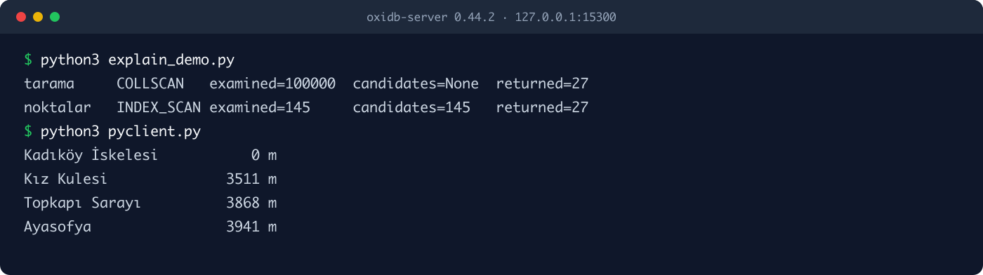
I ran the same kind of query through the official Python client too. The client does not have a create_geo_index helper yet, so I sent the raw command:
from oxidb import OxiDbClient

with OxiDbClient("127.0.0.1", 15300) as db:
    # The Python client has no create_geo_index helper yet; send the raw command
    db._checked({"cmd": "create_geo_index", "collection": "yerler", "field": "konum"})
    yakin = db.aggregate("yerler", [
        {"$geoNear": {"near": [29.0221, 40.9926], "key": "konum",
                      "distanceField": "m", "maxDistance": 4000}},
        {"$project": {"_id": 0, "ad": 1, "m": 1}},
    ])
    for d in yakin:
        print(f'{d["ad"]:<20} {d["m"]:>7.0f} m')
Kadıköy İskelesi 0 m
Kız Kulesi 3511 m
Topkapı Sarayı 3868 m
Ayasofya 3941 mRefusing shapes it cannot answer correctly
The easiest mistake in geo code is answering a shape "approximately" and telling nobody. OxiDB's rule is simple: a query I cannot answer correctly is refused by name. A wrong result list is far more expensive than an error message, because nobody notices it.
{"konum": {"$geoWithin": {"$center": [[28.98, 41.0], 0.02]}}}invalid query: $geoWithin $center is not supported - use $centerSphere (spherical), $box, or $geometry PolygonMongoDB's $center is a planar circle with a radius in degrees. At latitude 41, one degree of longitude is about 84 km and one degree of latitude about 111 km, so the "circle" is really an ellipse. Silently treating it as $centerSphere, or computing it on the plane, would both set the wrong expectations. Legacy $polygon is refused for the same reason:
invalid query: $geoWithin $polygon is not supported - use $centerSphere (spherical), $box, or $geometry PolygonA polygon spanning more than 180 degrees of longitude is refused too. Once a ring wraps half the globe, which side of it is "inside" becomes ambiguous on the plane:
{"konum": {"$geoWithin": {"$geometry": {"type": "Polygon",
  "coordinates": [[[-100, 0], [100, 0], [100, 10], [-100, 10], [-100, 0]]]}}}}
invalid query: Polygon spanning more than 180° of longitude is ambiguous - split it at the antimeridianA few more refusals, all real responses from the server:
swapped $box corners:  invalid query: $box corners must be [min, max] (no antimeridian wrap)
3-element point:       invalid query: expected a point ([lon, lat], GeoJSON Point, or {lon, lat}), got [41.0,28.9,1]
negative distance:     invalid query: $maxDistance must be a non-negative number of meters
LineString region:     invalid query: $geoWithin $geometry supports Polygon, got Some("LineString") - use $centerSphere for circles
(I wrote the long dash in the server's error messages as a plain hyphen here; the rest of the text is exactly what the server returned.)
Note the asymmetry: a broken point in a document is a non-match, a broken point in a query is an error. Documents are schemaless and can be messy; but you wrote the query, and a mistake in it is most likely a bug.
The geohash index: generous, never wrong
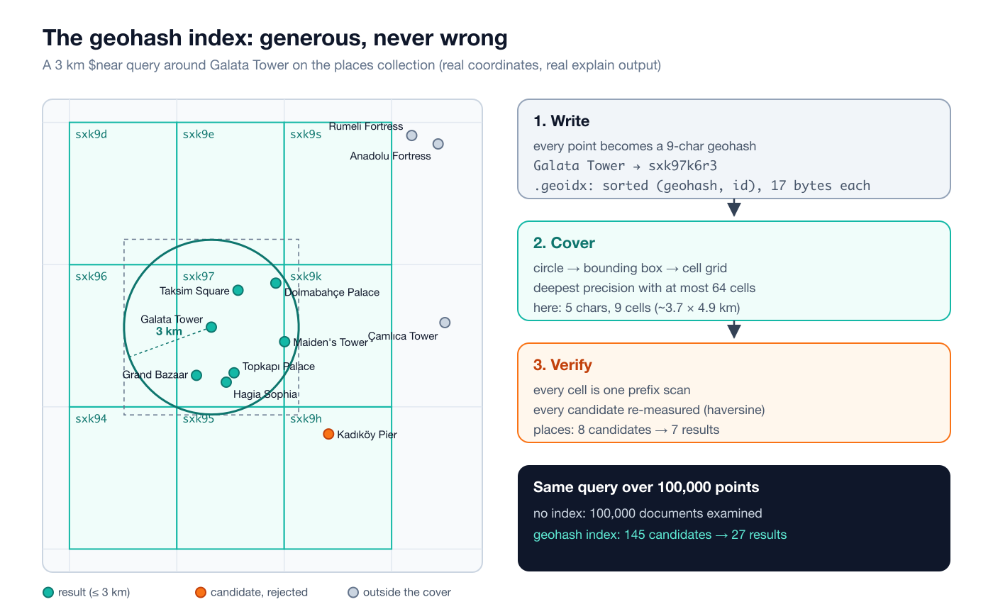
Now for the inside. A geohash is a classic encoding that turns a point into a short string by halving the world over and over. Longitude and latitude bits are interleaved (bit 0 longitude, bit 1 latitude, ...) and every 5 bits become one base32 character. The property that matters: geohashes that share a prefix lie in the same rectangular cell. Every point starting with sxk97 is inside the sxk97 cell.
The write side
Each indexed point becomes a fixed-precision 9-character geohash. Nine characters means cells of roughly 4.8 m × 4.8 m. Galata Tower is sxk97k6r3, Hagia Sophia sxk973qsr. The index is a sorted table of (geohash, document id) pairs: a BTreeMap<String, BTreeSet<DocumentId>> in memory and a .geoidx file on disk.
The .geoidx format is deliberately simple: the magic bytes OXGE, a 4-byte version, an 8-byte entry count, then fixed-width entries. Each entry is a 9-byte ASCII geohash and an 8-byte little-endian document id: 17 bytes. The fixed width follows from every geohash being exactly 9 characters, and it makes a prefix scan as simple as "binary-search the lower bound, walk while the prefix matches". On my test server the file for a 100,000-point collection was exactly 1,700,016 bytes: a 16-byte header plus 100,000 × 17. The places collection's file has 14 entries, because the café without a location is not in the index:
00000000: 4f58 4745 0100 0000 0e00 0000 0000 0000  OXGE............
00000010: 7378 6b36 7933 6271 700e 0000 0000 0000  sxk6y3bqp.......
00000020: 0073 786b 3871 7475 7831 0c00 0000 0000  .sxk8qtux1......
The query side: the cover
When a query arrives, I first turn its shape (circle, box or polygon) into a bounding box. Circles need some care: meters per degree of longitude shrink with latitude, so I use the widest latitude the circle reaches, which guarantees the box never undershoots. Then I try precisions from 9 downward and pick the deepest one whose cell grid covers the box in at most 64 cells. To find the cells I do no neighbor-table arithmetic; I lay a cell-sized grid of sample points over the box and geohash each one. That sidesteps the well-known traps of geohash neighbor computation entirely.
For 3 km around Galata Tower the result is 9 cells at precision 5: sxk94, sxk95, sxk96, sxk97, sxk9d, sxk9e, sxk9h, sxk9k, sxk9s. Precision 6 would have needed 88 cells, over the limit of 64. Each cell is one prefix scan of the index.
Verification: the index only nominates
This is the most important part of the design. The index only nominates candidates. Every candidate from the cells is checked again against the real predicate on the document itself (haversine distance, box test or polygon test). The cover may be generous and bring in extra candidates; it can never be wrong, because the document, not the index, has the last word.
You can see it with explain:
{"cmd": "explain", "inner": {"cmd": "find", "collection": "yerler", "query": {"konum": {"$near": {
  "$geometry": {"type": "Point", "coordinates": [28.9741, 41.0256]}, "$maxDistance": 3000}}}}}
{"ok": true, "data": {"strategy": "INDEX_SCAN", "index_used": "(range/in conditions)", "collection_docs": 15,
"candidates": 8, "examined": 8, "returned": 7, "post_filter": true, "post_filter_ops": [], "sort": "none",
"duration_ms": 0.005}}8 candidates, 7 results. The rejected candidate is the Kadıköy pier: it sits in cell sxk9h, inside the cover, but it is more than 3 km from Galata Tower. The index nominated it, verification threw it out.
This "the index is a hint, not the truth" contract matters even more in disk mode. In disk-first collections, the default since 0.38, the index has two layers: a sorted .geoidx base opened with mmap, and a small in-memory overlay of writes since the last persist. When a document moves or is deleted, its old base entry goes into a dead set; queries skip it, and at the next persist tick the base and overlay are merged into a fresh file that atomically replaces the old one. Suppose a stale entry slipped through somehow: the document would fail verification, so the result would still be correct. After a clean shutdown, opening is instant: no document scan, just an mmap. The file is checked on open as well: a wrong magic, wrong version or truncated file is refused and the index is rebuilt from the documents. After crash recovery it is rebuilt too. In-RAM collections (started with OXIDB_DISK_FIRST=0) persist only the index definition, and the index is rebuilt with one document scan at open.
I restarted the server and checked that the index was still there and produced the same plan (same 145 candidates, same 27 results). I also checked that the index follows updates: moving Topkapı Palace to Ankara's coordinates with $set dropped it from the 1.5 km-around-Hagia-Sophia query, and moving it back brought it back.
How much does it matter?
I inserted 100,000 random points over the Marmara region (longitude 26 to 31, latitude 39.5 to 42) and ran the same queries on the same data with and without the index. Measured on an Apple M4 Mac against the local server:
| Query (100,000 points) | No index | Geohash index |
|---|---|---|
3 km $near around Galata: documents examined | 100,000 | 145 candidates |
| Results | 27 | 27 |
| Median time measured from the client (20 runs) | 40.9 ms | 0.084 ms |
10 km $geoWithin around Hagia Sophia: documents examined | 100,000 | 527 candidates |
| Results | 270 | 270 |
| Median time measured from the client (20 runs) | 34.0 ms | 0.224 ms |
Times were measured from Python over TCP, JSON decoding included. The rows that really matter are the "Results" rows: the answer is the same with and without the index. That is exactly what the project's tests (tests/geo_queries.rs) check: an indexed query must return the same result as the unindexed scan across inserts, updates, deletes and a reopen.
The cover has a floor too. If a shape is so large that even the coarsest precision cannot cover it in 64 cells (half the planet, say), the cover returns "no restriction" and the query falls back to a full scan. The same goes for $near without a distance bound: every document is a candidate, then they are all sorted. Slow, but an honest plan.
Graph queries
The geo side answers "where?", the graph side answers "connected to what?". There is no separate graph data model in OxiDB: nodes are ordinary documents, and edges are either a reference field in a document (an array of ids, say) or documents in a separate edge collection. Two stages cover it: $graphLookup (reachability, BFS) and $shortestPath (shortest path, Dijkstra).
For the examples I built a small flight network: 11 airports in Turkey and 22 routes. Airport coordinates are real, and edge weights are the great-circle distances computed from those coordinates (km). The routes themselves are not real schedules, just an example network I picked.
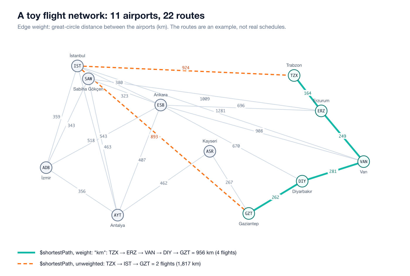
There are two collections. havalimanlari ("airports") holds the nodes, each with its neighbors' codes in an array (baglanti, "connections"); ucuslar ("flights") is the edge collection:
{"cmd": "find_one", "collection": "havalimanlari", "query": {"kod": "VAN"}}
{"ok": true, "data": {"kod": "VAN", "ad": "Van Ferit Melen", "konum": [43.3323, 38.4682],
  "baglanti": ["DIY", "ERZ", "ESB", "IST"], "_id": 8, "_version": 1}}
{"from": "TZX", "to": "ERZ", "km": 164}
{"from": "ERZ", "to": "VAN", "km": 249}
{"from": "IST", "to": "TZX", "km": 924}I put ordinary indexes on the connection fields: havalimanlari.kod, ucuslar.from and ucuslar.to. Why that matters will be clear in a moment.
$graphLookup: breadth-first search
$graphLookup is the same stage as in MongoDB: start from the startWith values, find documents whose connectToField equals them, then continue from their connectFromField values. "Where can I fly from Van with at most one connection?" (aktarma means "connection"):
{"cmd": "aggregate", "collection": "havalimanlari", "pipeline": [
  {"$match": {"kod": "VAN"}},
  {"$graphLookup": {"from": "havalimanlari", "startWith": "$baglanti",
     "connectFromField": "baglanti", "connectToField": "kod",
     "as": "erisilen", "depthField": "aktarma", "maxDepth": 1}},
  {"$unwind": "$erisilen"},
  {"$project": {"_id": 0, "kod": "$erisilen.kod", "aktarma": "$erisilen.aktarma"}},
  {"$sort": {"aktarma": 1, "kod": 1}}
]}
{"ok": true, "data": [
{"kod": "DIY", "aktarma": 0}, {"kod": "ERZ", "aktarma": 0}, {"kod": "ESB", "aktarma": 0}, {"kod": "IST", "aktarma": 0},
{"kod": "ADB", "aktarma": 1}, {"kod": "AYT", "aktarma": 1}, {"kod": "GZT", "aktarma": 1},
{"kod": "SAW", "aktarma": 1}, {"kod": "TZX", "aktarma": 1}, {"kod": "VAN", "aktarma": 1}
]}maxDepth: 0 returns only the direct flights (DIY, ERZ, ESB, IST). Without maxDepth the search runs until nothing new turns up and returns 11 documents; Kayseri (ASR) arrives in round 2. Note that VAN itself shows up in round 1: you can fly Van to Ankara and back, so VAN really is reachable. MongoDB behaves the same way; if you do not want the start document, filter it out afterwards.
Inside: one $in per round
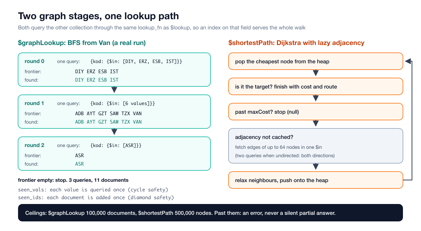
The most important property of $graphLookup is that every BFS round is one query. All frontier values of a round go into a single {connectToField: {$in: [...]}} query (wrapped in $and with restrictSearchWithMatch when given). That query goes through the same lookup_fn that $lookup uses, so an ordinary index on connectToField serves the whole walk. In the Van example the entire search is 3 queries: 4 values in round 0, 6 in round 1, 1 in round 2. In round 3 the frontier is empty and the search stops. A naive implementation issuing one query per node would have sent 11 queries for the same work; on large graphs the difference is measured in thousands.
Cycle safety comes from two separate sets, and each has its own job:
seen_vals: connection values already queried. A value is queried at most once. Without this set, a cycle (A follows B, B follows C, C follows A) would be re-queried forever.seen_ids: document ids already collected. A document appears in the result at most once. Without this set, a diamond (A→B→D and A→C→D) would return D twice.
I tried it on a tiny follow graph: ayşe follows mehmet, mehmet follows zeynep, zeynep follows both ayşe and can. There is a cycle:
{"cmd": "aggregate", "collection": "takip", "pipeline": [
  {"$match": {"kisi": "ayse"}},
  {"$graphLookup": {"from": "takip", "startWith": "$takip", "connectFromField": "takip",
     "connectToField": "kisi", "as": "ag", "depthField": "d"}},
  {"$unwind": "$ag"},
  {"$project": {"_id": 0, "kisi": "$ag.kisi", "d": "$ag.d"}}
]}
{"ok": true, "data": [{"kisi": "mehmet", "d": 0}, {"kisi": "zeynep", "d": 1}, {"kisi": "can", "d": 2}, {"kisi": "ayse", "d": 2}]}The search terminates and everyone appears once.
Pruning: restrictSearchWithMatch
restrictSearchWithMatch is applied during the traversal, not at the end. A document that fails the filter is dropped from the result and also stops being a door the search can continue through. "Where can I reach from Trabzon without connecting through Istanbul or Ankara?":
{"$graphLookup": {"from": "havalimanlari", "startWith": "$baglanti",
   "connectFromField": "baglanti", "connectToField": "kod", "as": "erisilen", "depthField": "aktarma",
   "restrictSearchWithMatch": {"kod": {"$nin": ["IST", "SAW", "ESB"]}}}}
{"ok": true, "data": [
{"kod": "ERZ", "aktarma": 0}, {"kod": "TZX", "aktarma": 1}, {"kod": "VAN", "aktarma": 1},
{"kod": "DIY", "aktarma": 2}, {"kod": "GZT", "aktarma": 3}, {"kod": "ASR", "aktarma": 4},
{"kod": "AYT", "aktarma": 5}, {"kod": "ADB", "aktarma": 6}
]}Only via Erzurum, east and then south, reaching Izmir after 6 connections. The filter is also parsed once when the stage is built, so a broken filter fails at pipeline construction, not on the first traversal round. Same for maxDepth: passing -1 gets you invalid pipeline: $graphLookup maxDepth must be a non-negative integer right away.
A practical note: startWith and connectFromField can be arrays (each element enters the frontier as its own value), but matching on connectToField is equality. In the target documents connectToField should hold a scalar. That is why I kept the neighbor list in the baglanti array and the matched field in the scalar kod.
Ceilings that err loudly
A graph can turn out much bigger than you expected. In a social network, "followers of followers" can reach millions in two hops. $graphLookup has a ceiling of 100,000 documents per input document. Past it, it does not return a silent partial result, it returns an error. A partial answer is a wrong answer that looks right.
To try it I created a single account with 100,001 followers:
{"cmd": "aggregate", "collection": "yildiz", "pipeline": [
  {"$match": {"kullanici": "merkez"}},
  {"$graphLookup": {"from": "yildiz", "startWith": "$kullanici", "connectFromField": "kullanici",
     "connectToField": "takip", "as": "takipciler"}},
  {"$project": {"_id": 0, "n": {"$size": "$takipciler"}}}
]}
invalid pipeline: $graphLookup found more than 100000 documents for one input document - narrow the traversal with maxDepth or restrictSearchWithMatch(The real message has some extra spaces left over from a line continuation in the source; I collapsed them to single spaces here. A small cosmetic flaw.) The error came back in about 156 ms; the ceiling kicks in long before an out-of-memory would. Adding restrictSearchWithMatch: {"kullanici": {"$in": ["u1", "u2", "u3"]}} to the same query returned {"n": 3}.
$shortestPath: Dijkstra over an edge collection
$shortestPath is not a MongoDB stage; it is an addition that deliberately walks into graph-database territory. For each input document it evaluates the source and target expressions and runs Dijkstra over the edges in the from collection. Each edge is a document of the form {edgeFrom: node, edgeTo: node, weight: number}.
First, unweighted, which minimizes the number of flights: Trabzon to Gaziantep (rota is "route", maliyet is "cost").
{"$shortestPath": {"from": "ucuslar", "source": "$kod", "target": "GZT",
   "edgeFrom": "from", "edgeTo": "to", "undirected": true, "as": "rota", "costField": "maliyet"}}
{"ok": true, "data": [{"kod": "TZX", "maliyet": 2.0, "rota": [
{"from": "IST", "to": "TZX", "km": 924}, {"from": "IST", "to": "GZT", "km": 893}]}]}Two flights, but 1,817 km via Istanbul. Now add weight: "km":
{"$shortestPath": {"from": "ucuslar", "source": "$kod", "target": "GZT",
   "edgeFrom": "from", "edgeTo": "to", "undirected": true, "as": "rota", "costField": "maliyet",
   "weight": "km"}}
{"ok": true, "data": [{"kod": "TZX", "maliyet": 956.0, "rota": [
{"from": "TZX", "to": "ERZ", "km": 164}, {"from": "ERZ", "to": "VAN", "km": 249},
{"from": "DIY", "to": "VAN", "km": 281}, {"from": "GZT", "to": "DIY", "km": 262}]}]}Four flights but only 956 km: Trabzon, Erzurum, Van, Diyarbakır, Gaziantep. The rota array lists the edge documents from source to target in order. With undirected: true, edges can be used in either direction, but the documents come back as stored; that is why the {"from": "DIY", "to": "VAN"} edge looks the way it does even though the route used it from VAN to DIY. You read the direction off the sequence.
The other parameters:
restrictSearchWithMatch: a filter applied to edges. The shortest route from Izmir to Van goes via Ankara, 1,451 km (ADB, ESB, VAN). Excluding Ankara's edges with{"from": {"$nin": ["ESB"]}, "to": {"$nin": ["ESB"]}}turns it into 1,601 km via Sabiha Gökçen and Erzurum.maxCost: the search stops once the cost exceeds this value. The same Izmir to Van query withmaxCost: 1200returned{"maliyet": null, "rota": []}. Since the heap always yields the cheapest node, once the top of the heap is past the bound everything else is too; stopping is safe.- Without
undirected(the default isfalse), edges are only usable in their stored direction. My network has no directed path from Trabzon to Gaziantep, so the answer ismaliyet: null. - Source equal to target is not "unreachable" but a zero-length path:
ISTtoISTgivesmaliyet: 0.0,rota: [].
Inside: lazy adjacency
Dijkstra itself is textbook and the settle order is never compromised: the heap always yields the cheapest unsettled node. What is batched is the data fetching. When the cheapest node's adjacency is not cached yet, it is grouped with up to 63 other heap nodes whose adjacency has not been fetched, and all their edges come back in one $in query (two when undirected, one per direction). That query also goes through the same lookup_fn as $lookup and $graphLookup, so indexes on edgeFrom and edgeTo serve the search. Once fetched, an adjacency stays cached.
"Lazy" is the key word: the edge collection is never loaded into memory wholesale. Only the adjacency of nodes the search actually touches is fetched. If the target is close, even an edge collection with millions of edges costs just a few queries.
Dijkstra's correctness depends on non-negative weights, and rather than silently assuming that, I check it:
invalid pipeline: $shortestPath: negative or non-finite weight -2 - Dijkstra requires non-negative weightsAn edge without a numeric weight is an error too:
invalid pipeline: $shortestPath: edge has no numeric 'ucret' weight: {"from":"TZX","to":"ERZ","km":164,"_id":21,"_version":1}So is a negative maxCost ($shortestPath maxCost must be a non-negative number). And like $graphLookup it has a ceiling: 500,000 settled nodes. Past it, an error again, with a message that tells you what to do: bound the search with maxCost or restrictSearchWithMatch. I did not build a 500,000-node graph to trigger this one separately; the value is in the source (MAX_SETTLED).
Limits and honest trade-offs
- Points only. You cannot store lines (LineString) or polygons in documents and ask "does this road cross this region?". Polygons exist on the query side, not on the data side. That is a conscious v1 scope: most location data is points (users, vehicles, shops, sensors).
- Polygons are planar. Correct at geofence scale, not at continent scale. Polygons wider than 180 degrees of longitude are refused;
$boxdoes not wrap the antimeridian. - One geo predicate per query uses the index. If a query has several geo predicates, the first one produces candidates and the rest are checked during verification. Combining with an ordinary index works well, though: after I also indexed
tur, explain for{"tur": "kule", "konum": {"$near": ... 3 km}}showed 2 candidates; the two indexes' candidate sets were intersected. - Unbounded
$nearmeans a full scan. Without$maxDistancethe index cannot compute a cover; every document becomes a candidate and is then sorted. On large collections always give a distance bound, or use it with alimit. $nearsorts in memory. The sort happens in memory after the candidate set has been verified. Negligible when the cover is small, not for an unbounded query.- Graph stages run per input document.
$graphLookupafter a$matchthat returns 1,000 documents means 1,000 separate BFS runs. Narrow first. $shortestPathneeds non-negative weights. There is no Bellman-Ford for negative edges; you get an error.- One shortest path. If several paths tie, one is returned; there is no k-shortest-paths or all-paths.
How it fits with the rest of OxiDB
Geo and graph queries are not a separate engine but part of the document engine's query language. So they compose naturally with everything else: $group after $geoNear, $lookup after $graphLookup, in the same pipeline. A location is ultimately an ordinary field; updates, deletes and index maintenance go down the same path as the rest of the document engine.
The same engine also compiles to WebAssembly. The geo globe demo is that, live: populated places from GeoNames are loaded into OxiDB in a browser tab, clicking the globe runs a real $near, dragging the slider runs $geoWithin with $centerSphere, and route mode snaps two clicks to the road graph with $near and runs $shortestPath (Dijkstra) as one aggregation inside the tab. No server.
If you prefer to talk Redis, the OxiMem side has RESP GEO commands such as GEOADD, GEOSEARCH and GEODIST; there I followed Redis's own design (a GEO key is a sorted set scored by a 52-bit geohash). For time-stamped data see the time series engine, and if you would rather write queries in SQL, the SQL engine. Similarity graphs and the like are a topic for the recommendation engine post.
Try it
OxiDB is a single binary. The easiest way is to grab the build for your platform from the GitHub releases page, or use the Docker image. Start the server, index a location field with create_geo_index, and try the queries above. Graphs need no setup at all: your documents already are nodes and your references already are edges. Just remember to index the connection fields; the speed of $graphLookup and $shortestPath depends almost entirely on that.
Going forward I will keep the rule from this post: when I cannot answer a query correctly, you get a clear error instead of an approximate answer.