Full-text and vector search in OxiDB
OxiDB's search layer: BM25 ranking, Snowball stemming in 18 languages with Turkish examples, highlighted snippets, searching inside PDF/DOCX/XLSX files, an mmap'd inverted index, k-NN with HNSW and measured recall.

Once a document is in OxiDB you want to find it by more than field equality: by the words inside it, and by other documents that mean something similar. I did not want that to require a separate Elasticsearch cluster or a separate vector database, so I built both into the same process. Full-text search in OxiDB has BM25 ranking, Snowball stemming, <mark> highlighted snippets and text extraction from PDF, DOCX and XLSX. Vector search does k-NN with cosine, Euclidean or dot product, scanning exactly on small collections and switching to HNSW on large ones. This post walks through how to use both, how they work inside and where they fall short, using real sessions. Every output shown here comes from an OxiDB 0.44.2 server I ran for this post on my own machine (Apple M4, local).
This is the second post in the series. The document model, query language and index types are covered in the document engine post; here I focus on the search layer built on top of them.
Two kinds of search, one process
"Search" means two different things in OxiDB:
| Full-text search | Vector search | |
|---|---|---|
| Finds | Documents containing the query words (reduced to their stems) | The k vectors closest to the query vector |
| Index | create_text_index (collections), automatic (blobs/files) | create_vector_index |
| Ranking | BM25 (_score) | Distance (_distance) plus a 0-1 similarity (_similarity) |
| Command | text_search, search | vector_search |
| On disk | .mtidx (mmap'd inverted index) | not persisted in 0.44.2 (see below) |
Full-text search itself has two faces. For collection documents, the string fields you pick with create_text_index are indexed and searched with text_search. Files you put into the blob store (the S3-compatible object store) are converted to text by content type, go into a separate global index and are searched with search. Both use the same tokenizer and the same BM25 code.
There is no flag to turn search on: if the document engine is running (the default), the search commands are there. Language and BM25 settings are environment variables. For this post I ran two servers, one with Turkish stemming and one with English:
OXIDB_ADDR=127.0.0.1:15200 OXIDB_DATA=./data-tr OXIDB_FTS_LANG=tr \
OXIDB_S3_PORT=15210 OXIDB_HTTP_PORT=15220 ./oxidb-server
At startup the server prints the configuration in one line:
FTS: lang=turkish k1=1.2 b=0.75 (BM25)Full-text search on a collection
Creating the index
I inserted a handful of Turkish documents and built a text index over two fields. The native protocol is length-prefixed JSON; these requests went over it and the responses are exactly what the server returned:
{"cmd": "insert_many", "collection": "yazilar", "docs": [
  {"baslik": "Kütüphanedeki eski kitaplar", "metin": "Kütüphanedeki eski kitaplar yeniden düzenlendi, raflar alfabetik sıraya kondu."},
  {"baslik": "Bir romana dönüş", "metin": "Bu kitabı okumadan önce yazarın ilk romanına bakmanızı öneririm."},
  {"baslik": "Haritada edebiyat", "metin": "Kitaplarda geçen yer adlarını tek tek haritaya döktüm."},
  {"baslik": "Rust ile veritabanı yazmak", "metin": "Kendi veritabanımı yazarken tuttuğum notlar: sayfa yapısı, WAL ve indeksler."},
  {"baslik": "Kahve demlemenin altı yolu", "metin": "French press, V60 ve moka pot ile kahve demlemek üzerine kısa bir rehber."},
  {"baslik": "Çocuklar için masallar", "metin": "Çocuklar için resimli masal kitapları seçerken dikkat ettiğim şeyler."},
  {"baslik": "Veritabanlarında indeks seçimi", "metin": "Veritabanlarında hangi alana indeks koymalı? Seçicilik ve sorgu planı."},
  {"baslik": "Kitapçıda bir öğleden sonra", "metin": "Sahaftan aldığım kitapların listesi ve kısa notlarım."}
]}
{"cmd": "create_text_index", "collection": "yazilar", "fields": ["baslik", "metin"]}
{"cmd": "list_indexes", "collection": "yazilar"}
{"ok": true, "data": [1, 2, 3, 4, 5, 6, 7, 8]}
{"ok": true, "data": "text index created"}
{"ok": true, "data": [{"name": "_text", "index_type": "text", "fields": ["baslik", "metin"], "unique": false}]}Existing documents are backfilled when the index is created. There is one text index per collection, always named _text; it can span several fields, and field paths can use dot notation (meta.summary). Arrays of strings are read too; numbers and other types are skipped.
Turkish stemming
What I wanted to see first is that Turkish suffixes do not break search. Turkish is agglutinative: "kitap" (book) becomes "kitaplar" (books), "kitaplarda" (in the books), "kitabı" (the book, accusative, with the p softened to b). A search for any of them should find the others:
== kitap ==
0.6557  _id=1  Kütüphanedeki eski kitaplar
0.5500  _id=8  Kitapçıda bir öğleden sonra
0.5276  _id=2  Bir romana dönüş
0.5069  _id=3  Haritada edebiyat
0.5069  _id=6  Çocuklar için masallar

== kitaplar ==
0.6557  _id=1  Kütüphanedeki eski kitaplar
...
== kitaplarda ==
0.6557  _id=1  Kütüphanedeki eski kitaplar
...
All three queries return the same five documents with identical scores, because they reduce to the same stem. The b/p softening in "kitabı" is handled by Snowball's Turkish rules. A condensed run of the same experiment:
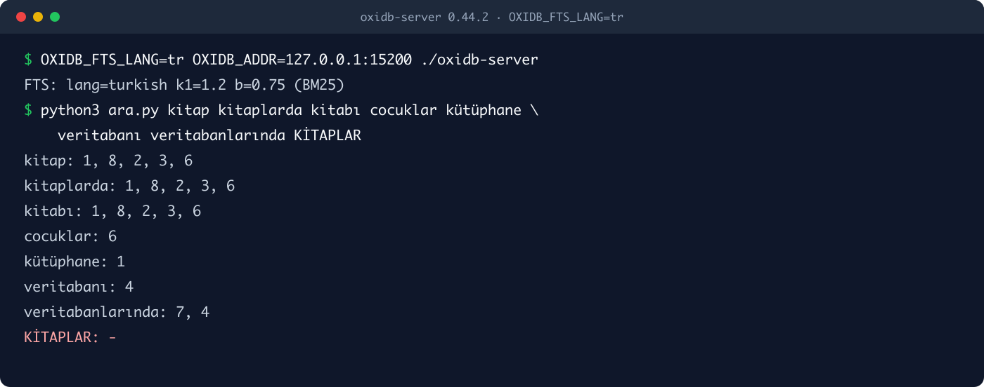
The document numbers: 1 "eski kitaplar", 2 "Bu kitabı", 3 "Kitaplarda geçen", 6 "masal kitapları", 8 "kitapların listesi", 4 "veritabanı, veritabanımı" (database, my database), 7 "Veritabanlarında" (in databases).
Two things stand out. Typing cocuklar without Turkish characters still finds "Çocuklar" (children), because the tokenizer strips accents before stemming (ç→c, ş→s, ğ→g, ı→i, ö→o, ü→u). It is a nice side effect for users without a Turkish keyboard. The same session also shows the cost of that choice; I come back to it under limits.
How a query is interpreted
text_search combines query terms with OR: a document matching any term is in the result, and documents matching more of them score higher. A search for eski kitaplar ("old books") puts the single document containing "eski" on top and lists the ones that only contain "kitap" after it:
== eski kitaplar == 1:3.041; 8:0.550; 2:0.528; 3:0.507; 6:0.507There is no quoted phrase search, no AND/NOT operators and no per-field boosting. I kept it simple on purpose: the query goes through the same tokenizer as the documents and the term contributions are summed. Ties are broken by _id; I added that later, because when ties came out in hash map iteration order, pagination returned different pages run to run.
Highlighted snippets: <mark>
Pass highlight and every result carries short <mark>-tagged snippets from each indexed string field. Since it uses the same tokenizer, a query for kitaplar also marks kitabı. This time I used the REST interface with plain curl:
curl -s -X POST http://127.0.0.1:15220/api/yazilar/text_search \
  -H 'Content-Type: application/json' \
  -d '{"query":"çocuk kitapları","limit":2,"highlight":{"snippet_chars":50,"max_snippets":1}}'
[
{
"_id": 6,
"_version": 1,
"baslik": "Çocuklar için masallar",
"metin": "Çocuklar için resimli masal kitapları seçerken dikkat ettiğim şeyler.",
"_score": 3.0199245077882484,
"_highlights": {
"baslik": ["<mark>Çocuklar</mark> için masallar"],
"metin": ["<mark>Çocuklar</mark> için resimli masal <mark>kitapları</mark> seçerken dikkat ettiği"]
}
},
{
"_id": 1,
"_version": 1,
"baslik": "Kütüphanedeki eski kitaplar",
"metin": "Kütüphanedeki eski kitaplar yeniden düzenlendi, raflar alfabetik sıraya kondu.",
"_score": 0.6557111258304198,
"_highlights": {
"baslik": ["Kütüphanedeki eski <mark>kitaplar</mark>"],
"metin": ["Kütüphanedeki eski <mark>kitaplar</mark> yeniden düzenlendi, raf"]
}
}
]highlight: true uses the defaults (80 characters, at most 3 snippets); an object lets you set snippet_chars and max_snippets. Snippets are ordered by match density. Cut points snap to UTF-8 character boundaries: slicing a Rust string in the middle of a Turkish letter is a panic, so I test this with Turkish text specifically. The tags can be changed at the library level (highlight_with_tags); the server uses <mark>. Highlighting re-tokenizes the text of every result, so it is not free: it only happens on request and scans at most the first 256 KB per field (OXIDB_FTS_MAX_HIGHLIGHT_BYTES).
Updates and deletes show up immediately
The collection text index is updated inside the write path, so the moment an update returns, search sees the new text:
text_search 'moka' -> 5:1.595
>>> {"cmd": "update", "collection": "yazilar", "query": {"_id": 5}, "update": {"$set": {"metin": "Moka pot ile kahve: bir kitaptan öğrendiğim üç püf noktası."}}}
{"ok": true, "data": {"modified": 1}}
text_search 'moka' -> 5:1.210
text_search 'kitap' -> 1:0.430, 8:0.361, 2:0.346, 3:0.332, 6:0.332, 5:0.307
>>> {"cmd": "delete", "collection": "yazilar", "query": {"_id": 5}}
{"ok": true, "data": {"deleted": 1}}
text_search 'moka' ->
Once document 5 contained "kitaptan" ("from a book") it joined the kitap results, and every other document's score dropped: more documents now contain the term, so its IDF went down. After the delete, moka returns nothing.
BM25: where the scores come from
The first version used TF-IDF. It had two problems: long documents won just by being long, and a document repeating a word ten times got ten times the score. In 0.25.9 I switched to BM25 with the Lucene/Elasticsearch defaults, k1 = 1.2 and b = 0.75.
A term's contribution to a document's score:
idf   = ln( (N - df + 0.5) / (df + 0.5) + 1 )
norm  = 1 - b + b * (dl / avgdl)
score = idf * tf * (k1 + 1) / (tf + k1 * norm)
N is the number of documents, df the number containing the term, tf the term's frequency in this document, dl the document's token count and avgdl the corpus average. For multi-term queries the contributions add up.
To see the behaviour, I set up three documents on the English server on purpose: an 8-token note mentioning "raft" twice, a 54-token text mentioning it once, and a 35-token document repeating it 13 times.
== raft ==
1.8004  _id=3  Raft raft raft
1.5453  _id=1  Raft in five minutes
0.5291  _id=2  Notes from a long week of operations
Thirteen repetitions earn only 16% more than two: that is k1 saturation. I recomputed the scores from the formula in Python (N=8, avgdl=18.5, df=3, idf=0.9445) and they match to four decimals: 1.5453, 0.5291, 1.8004.
Then I restarted the server with OXIDB_FTS_B=0, switching length normalization off:
FTS: lang=english k1=1.2 b=0 (BM25)
== raft (b=0) ==
1.9022  _id=3  Raft raft raft
1.2986  _id=1  Raft in five minutes
0.9445  _id=2  Notes from a long week of operations
The long document went from 0.53 to 0.94 and the short note dropped from 1.55 to 1.30. No reindex was needed: k1 and b are applied at query time, and the index only stores tf, dl and the total token count.
Settings
All FTS settings are read once at process start and cached (OnceLock), so changing them requires a restart:
| Variable | Default | What it does |
|---|---|---|
OXIDB_FTS_LANG | english | Snowball language: tr, de, fr, es, it, pt, ru, nl, da, fi, hu, no, ro, el, ar, sv, ta, en (18 languages) |
OXIDB_FTS_K1 | 1.2 | Term-frequency saturation (> 0) |
OXIDB_FTS_B | 0.75 | Length normalization (0 to 1) |
OXIDB_FTS_SCORE_CAP | 200000 | Max distinct documents one search scores; 0 = unbounded |
OXIDB_FTS_MAX_EXTRACT_BYTES | 4 MB | Max text extracted from one file; 0 = uncapped |
OXIDB_FTS_MAX_HIGHLIGHT_BYTES | 256 KB | Max text a highlight scans |
OXIDB_FTS_WORKERS | 1 | File indexing worker threads |
OXIDB_FTS_FLUSH_INTERVAL_MS | 1000 | How often the blob index is written to disk |
OXIDB_OCR_LANGS | eng | Tesseract languages, e.g. eng+tur (only with the ocr feature) |
OXIDB_OCR_PREPROCESS | on | Grayscale, 2x upscale and Otsu threshold before OCR |
One caveat: the index stores stemmed terms. If you change OXIDB_FTS_LANG on existing data, queries are stemmed with the new language while the index holds the old one's stems. After a language change, drop _text with drop_index and create the index again.
Searching inside files
When a file is written to the blob store (native put_object or an S3 PUT), the server puts it on an FTS queue. A worker thread reads the file, extracts text according to its content type and adds it to the global index. Supported types:
| Content type | How |
|---|---|
text/* | As is |
text/html, text/xml, application/xml | Tags stripped |
application/json | All string values collected recursively |
application/pdf | pdf_extract |
| DOCX | Text in word/document.xml |
| XLSX | Cell text in xl/sharedStrings.xml |
image/png, jpeg, tiff, bmp | Tesseract OCR, only when built with --features ocr |
I tried it with six files: an HTML meeting note, an XML product catalogue, a JSON settings file, a DOCX contract draft produced with macOS textutil, an XLSX stock list and a PDF invoice produced with cupsfilter, all with Turkish content. Five went in over the native protocol; the PDF went through the S3 interface with plain curl and no client library at all:
curl -s -i -X PUT --data-binary @fatura.pdf -H "Content-Type: application/pdf" \
  http://127.0.0.1:15210/belgeler/fatura.pdf
HTTP/1.1 200 OK
Server: OxiDB-S3
ETag: "a249de4c7ae443472e09ffd73baf6b86"(S3 authentication was off here, which is why an unsigned PUT was accepted. The S3 side is covered in detail in the S3 post.)
Since indexing is asynchronous, fts_status shows what happened: queue depth, what each worker is doing and how recent jobs ended:
{"cmd": "fts_status"}
queue_depth: 0, workers: [{"id": 0, "current": null}]
toplanti.html  indexed  0 ms
katalog.xml    indexed  0 ms
ayarlar.json   indexed  0 ms
sozlesme.docx  indexed  0 ms
stok.xlsx      skipped  "no extractor for content type"
fatura.pdf     indexed  3 ms
(The response is JSON; I flattened it into lines for reading.) The XLSX was skipped, and the reason is interesting. I had produced it with Python's openpyxl, which writes cell text inline instead of into sharedStrings.xml, and OxiDB's extractor only reads sharedStrings.xml. Files saved by Excel itself use the shared string table, so most real files are fine, but the message "no extractor for content type" is misleading here: there is an extractor, it just found no text. I repackaged the same table with a shared string table and uploaded it again to the same key over S3, and it was indexed; an overwrite drops the old entry from the index and adds the new one.
Searches:
== kitap ==      ayarlar.json:0.822; stok.xlsx:0.757; toplanti.html:0.612
== depozito ==   sozlesme.docx:1.426
== kahve ==      katalog.xml:1.221; stok.xlsx:1.124
== tedarikçi ==  stok.xlsx:1.682
== faturası ==   fatura.pdf:1.109
search supports highlighting too, but it costs more here: the index does not store text, so every hit's file is read again and its text re-extracted. That is why it only happens on request:
{"cmd": "search", "query": "kitaplar", "bucket": "belgeler", "limit": 5,
 "highlight": {"snippet_chars": 70, "max_snippets": 1}}
{"ok": true, "data": [
{"bucket": "belgeler", "key": "ayarlar.json", "score": 1.0502388364929411,
"highlights": ["OxiDB demo <mark>Kitap</mark> arşivi için arama ayarları tr e"]},
{"bucket": "belgeler", "key": "toplanti.html", "score": 0.7880432878539266,
"highlights": ["in indeksleme kuyruğu konuşuldu. <mark>Kitapların</mark> PDF sürümleri de aranabilir olac"]}
]}Defending against hostile files
Text extraction means parsing untrusted input. DOCX and XLSX are zip archives, and a 100 KB upload can inflate to gigabytes. So the zip readers stop pulling at four times the 4 MB text cap (Read::take) and the bomb is never fully inflated. That is not possible for PDF, because pdf_extract manages its own memory; I can truncate its output afterwards, but I cannot bound the library's internal memory from outside, and the code says so explicitly. Extractors can panic on malformed input, so every job runs inside catch_unwind: with a single worker, one panic used to silently stop file indexing for the rest of the process lifetime.
OCR
Text from images sits behind the ocr feature because it needs the Tesseract and Leptonica system libraries. The image is converted to grayscale, upscaled 2x and binarized with Otsu's method first, which makes a real difference on phone photos of documents. The repo's Dockerfile builds the server with --features cluster,ocr. The prebuilt macOS binary I used has no OCR: when I uploaded a PNG, fts_status honestly reported skipped: no extractor for content type.
Inside: how the inverted index is stored
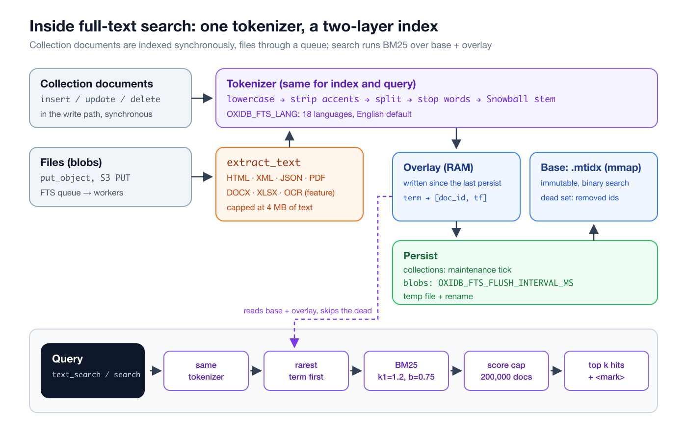
Tokenizer
Indexing and querying go through the same function: lowercase, strip accents, split on non-alphanumeric characters, drop one-letter fragments and stop words, stem with Snowball. The stop word list is the union of the English and Turkish lists and is always applied regardless of the language setting.
Collection index: overlay plus an mmap'd base
In the first version the collection text index lived entirely in RAM and was rebuilt by scanning the collection on every open. According to the project's own measurement (examples/fts_mem_bench.rs, 1 million documents with about 120 bytes of text each), that index took 1015 MB while the documents themselves took 38 MB. I first interned terms with Arc<str> to get it down to 785 MB, then gave the index a disk form.
The current model is the field indexes' .mfidx model applied to postings:
- Base (
<collection>.mtidx): an immutable file opened with mmap. A header (OXTImagic, version, fields, total token count), a fixed-stride doc table (doc_id u64, dl u32), postings (12 bytes each:doc_id u64, freq u32), a term table sorted by bytes, and the term strings. Both doc and term lookups are binary searches directly over the mmap. - Overlay: a small in-RAM index for documents written since the last persist.
- Dead set: the base cannot be edited, so ids of removed or re-indexed documents go into a set and search skips their base postings. It is the same idea as Lucene's deleted-docs bitmap.
The first bytes of the file from my run:
00000000: 4f58 5449 0100 0000 0200 0500 7469 746c  OXTI........titl
00000010: 6504 0062 6f64 7994 0000 0000 0000 0008  e..body.........
Persist happens at the periodic maintenance tick where documents are snapshotted: base and overlay are merged, the dead are dropped, and a new file is written. The write streams term by term; postings sit before the term table in the file, so each term's postings are appended straight to disk and only the vocabulary-sized term table waits in memory. The file is written under a temporary name and moved into place with rename, so a crash leaves the previous file in force. If the file is missing, short or corrupt at open, the collection is scanned and the index rebuilt. The same rebuild happens when crash recovery replayed WAL entries, because the disk index was written before the crash and does not know about the recovered records.
In the project's measurements after this change, at 1 million documents the resident index is 0 MB (mmap), the build peak is 265 MB with a persist every 200k documents, and a common-term search peaks at 7.3 MB and takes 35 ms.
I ran a smaller test on my machine: 200,000 documents of 12 random words each, with "coffee" in half of them, "curtain" in 5% and "emerald" in 0.1%. (This server was still running with b=0 from the previous experiment; that does not affect timing.)
N=200000: insert 2.1s, create_text_index 4.06s
'emerald'          hits(top10)=10  p50=0.11 ms  p95=0.20 ms
'curtain'          hits(top10)=10  p50=1.25 ms  p95=2.42 ms
'coffee'           hits(top10)=10  p50=8.80 ms  p95=11.22 ms
'coffee emerald'   hits(top10)=10  p50=8.81 ms  p95=10.73 ms
The times include the Python client's round trip. The .mtidx file came to 33 MB (about 2.7 million postings at 12 bytes).
Why there is a score cap
Term-at-a-time BM25 keeps a score entry for every matching document before limit applies. A term present in half a million documents means that many entries for one search; the project measured 25 MB per query at 500k matches and 51 MB at 1M. Multiplied by concurrent searches, that was an OOM. Now one search scores at most 200,000 distinct documents. The order is what makes this safe: terms are processed from rarest to most common, so every document matching a rare, informative term is scored before the budget fills, and what the cap cuts is the tail of the most common (least informative) term's list. Once at the cap, documents already scored keep accumulating; new ones are not admitted.
The blob index and batched writes
The file index uses the same model (_fts/index.mtidx) with two differences: documents are named by (bucket, key), so postings carry a 4-byte ordinal (8 bytes per posting), and each document records the byte size of its extracted text for per-bucket quota accounting. In the first version the index was a single index.json, and every added document rewrote the whole file: N² disk writes on bulk ingestion. Now workers only mark the index dirty, and a background flusher writes it at most once per OXIDB_FTS_FLUSH_INTERVAL_MS (1 second by default). A legacy index.json is migrated to the mmap format on first open and removed; a corrupt one is quarantined and the index starts empty, because FTS is derived data and must not block startup.
There is a consistency trade-off here: the collection index is current at write time, while the blob index lags a few milliseconds behind until the queue drains. A search right after put_object may not see the new file yet. That is exactly what fts_status is for.
Vector search
Vector search is for storing embeddings next to documents and asking "which documents are closest in meaning to this query". OxiDB does not produce embeddings; you compute the vector (with a model) and store it in a document field as an array of numbers.
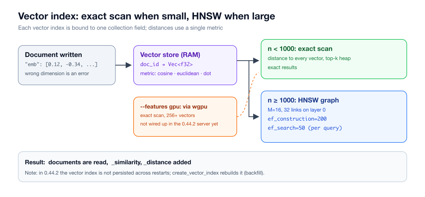
Index and query
I did not use an embedding model for this post. To show the mechanics I used hand-written four-dimensional vectors, where the dimensions stand for "databases", "search", "coffee" and "books":
{"cmd": "insert_many", "collection": "articles", "docs": [
  {"title": "B-tree page splits explained",       "emb": [0.9, 0.2, 0.0, 0.1]},
  {"title": "Building an inverted index",         "emb": [0.6, 0.9, 0.0, 0.1]},
  {"title": "BM25 by hand",                       "emb": [0.3, 1.0, 0.0, 0.2]},
  {"title": "HNSW graphs for embeddings",         "emb": [0.5, 0.8, 0.0, 0.0]},
  {"title": "Pour-over coffee ratios",            "emb": [0.0, 0.0, 1.0, 0.1]},
  {"title": "Coffee shops with good bookshelves", "emb": [0.0, 0.1, 0.7, 0.7]},
  {"title": "Second-hand books in Istanbul",      "emb": [0.0, 0.1, 0.1, 1.0]},
  {"title": "Reading list: database internals",   "emb": [0.8, 0.3, 0.0, 0.8]}
]}
{"cmd": "create_vector_index", "collection": "articles", "field": "emb", "dimension": 4, "metric": "cosine"}
{"cmd": "vector_search", "collection": "articles", "field": "emb", "vector": [0.7, 0.7, 0.0, 0.0], "limit": 3}
{"ok": true, "data": [
{"title": "Building an inverted index", "emb": [0.6, 0.9, 0.0, 0.1], "_id": 2, "_version": 1,
"_similarity": 0.9882084, "_distance": 0.023583233},
{"title": "HNSW graphs for embeddings", "emb": [0.5, 0.8, 0.0, 0.0], "_id": 4, "_version": 1,
"_similarity": 0.9871956, "_distance": 0.025608778},
{"title": "BM25 by hand", "emb": [0.3, 1.0, 0.0, 0.2], "_id": 3, "_version": 1,
"_similarity": 0.9323735, "_distance": 0.1352529}
]}A query vector like "books to read with coffee" ([0, 0, 0.6, 0.8]) lands in a completely different corner:
sim=0.9925  dist=0.0151  Coffee shops with good bookshelves
sim=0.9258  dist=0.1485  Second-hand books in Istanbul
sim=0.8383  dist=0.3234  Pour-over coffee ratios
sim=0.7734  dist=0.4532  Reading list: database internals
The rules are simple: each vector index is bound to one field (dot notation works), a collection can have several vector indexes on different fields, and existing documents are backfilled when the index is created. A vector with the wrong dimension is an error, a document without the field is skipped silently. Results come back as whole documents with _distance (lower is better) and _similarity (0 to 1, higher is better) added.
Three metrics, three different answers
The choice of metric really changes the result. To show it I put the same four points into three fields, indexed each with a different metric and queried with [1, 1]. B points the same way as A but is five times longer:
query = [1.0, 1.0]
-- cosine
   A [1.0, 1.0]   distance=-1.19209e-07 similarity=1.0000
   B [5.0, 5.0]   distance=0           similarity=1.0000
   C [1.2, 0.8]   distance=0.0194193   similarity=0.9903
   D [-1.0, 2.0]  distance=0.683772    similarity=0.6581
-- euclidean
   A [1.0, 1.0]   distance=0           similarity=1.0000
   C [1.2, 0.8]   distance=0.282843    similarity=0.7795
   D [-1.0, 2.0]  distance=2.23607     similarity=0.3090
   B [5.0, 5.0]   distance=5.65685     similarity=0.1502
-- dot_product
   B [5.0, 5.0]   distance=-10         similarity=0.0000
   A [1.0, 1.0]   distance=-2          similarity=0.1192
   C [1.2, 0.8]   distance=-2          similarity=0.1192
D [-1.0, 2.0] distance=-1 similarity=0.2689- cosine (
1 - cos) only looks at direction: A and B tie. It is the default and the right choice for text embeddings. The-1.19e-07for A is float rounding. - euclidean looks at actual distance: B drops to last.
- dot_product (
-a·b) rewards magnitude: B comes first. On normalized vectors it gives the same order as cosine and is cheaper.
Preparing this table, I caught a bug: with dot product the ranking is correct but _similarity is inverted. B, the best match, has similarity 0.0000 and D, the worst, has 0.2689. The code comment says "sigmoid(dot)", but it computes 1 / (1 + e^(-distance)), and since distance is already -dot, that is sigmoid(-dot). docs/vector-search.md describes yet another formula ((1 + d) / 2). Until I fix it, use _distance with dot product. list_indexes shows the metric as dotproduct; requests accept both dot_product and dotproduct, and an unrecognized metric name silently falls back to cosine.
Exact scan or HNSW
While the index has fewer than 1000 vectors, each query computes the distance to every vector and keeps the nearest k in a heap; the result is exact. At 1000 an HNSW (Hierarchical Navigable Small World) graph is built, and later inserts go into it incrementally. Parameters: M = 16 links (32 on layer 0), ef_construction = 200, and ef_search defaults to 50 and can be set per request. Removing a node cuts its links from its neighbours, the graph is rebuilt once more than 20% of its nodes are deleted, and if the count falls below 500 the graph is dropped and search goes back to exact scanning.
The docs claim ">95% recall" for HNSW. I wanted to measure it. I generated synthetic vectors clustered around 50 centres (closer to real embeddings than uniform noise), computed exact cosine results for 200 queries with numpy and compared them with the top 10 OxiDB returned:
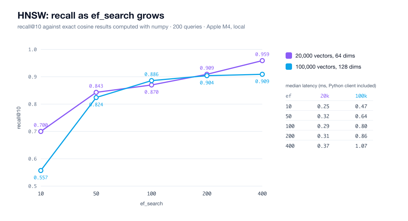
N=20000 D=64: insert 1.03s, create_vector_index 2.28s
ef_search=10   recall@10=0.700  latency p50=0.25 ms  p95=0.35 ms
ef_search=50   recall@10=0.843  latency p50=0.32 ms  p95=0.65 ms
ef_search=100  recall@10=0.870  latency p50=0.29 ms  p95=0.40 ms
ef_search=200  recall@10=0.909  latency p50=0.31 ms  p95=0.39 ms
ef_search=400  recall@10=0.959  latency p50=0.37 ms  p95=0.51 ms

N=100000 D=128: insert 9.92s, create_vector_index 34.45s
ef_search=10   recall@10=0.557  latency p50=0.47 ms  p95=0.54 ms
ef_search=50   recall@10=0.824  latency p50=0.64 ms  p95=0.74 ms
ef_search=100  recall@10=0.886  latency p50=0.80 ms  p95=1.11 ms
ef_search=200  recall@10=0.904  latency p50=0.86 ms  p95=0.97 ms
ef_search=400  recall@10=0.909  latency p50=1.07 ms  p95=1.31 ms
The honest result: on this data, the default ef_search=50 gives 82-84% recall, not 95%. At 20k vectors ef_search=400 reaches 96%; at 100k it plateaus around 91%, which means the limit there is graph quality, not search width. Latency stays around a millisecond either way (including the Python client round trip). My practical advice: if recall matters, pass ef_search of 200-400. If you need exact results, there is currently no way to force an exact scan above 1000 vectors; that threshold is hard-coded. In a 900-vector control run, recall was 1.000 at every ef_search, as expected.
GPU
Built with --features gpu, src/gpu.rs runs a WGSL compute shader through wgpu: three entry points for cosine, Euclidean and dot product, workgroups of 256, one GPU thread per stored vector computing its distance to the query, with the CPU picking the top k. Metal on macOS, Vulkan on Linux, DX12 on Windows. The design hands exact scans of 256 or more vectors to the GPU.
But reading the code for this post, I found that the 0.44.2 server initializes the GPU at startup, prints "GPU compute: enabled" and hands the handle to the engine, and the engine never passes it on to the collections' vector indexes (VectorIndex::set_gpu is not called anywhere). So in this release the GPU path is effectively not in use. The binary I used was built without the GPU feature anyway, so I did not measure anything on the GPU. Finishing that wiring is on my list.
Persistence: the vector index is lost on restart
docs/vector-search.md says the index is saved to .vidx files and restored at startup. That is true for the old Collection engine. On the B-tree collections the server uses today, the vector index is written neither to the index metadata nor to disk. After restarting the server:
>>> {"cmd": "list_indexes", "collection": "articles"}
{"ok": true, "data": []}
>>> {"cmd": "vector_search", "collection": "articles", "field": "emb", "vector": [0.7, 0.7, 0, 0], "limit": 2}
{"ok": false, "error": "invalid query: no vector index on field 'emb'; create one with create_vector_index"}
After the same restart, the text index came back from .mtidx instantly with identical scores. No data is lost, because the vectors live in the documents: create_vector_index is idempotent and rebuilds from them. But at 100k × 128 dimensions that takes 34 seconds. Calling create_vector_index when your application starts is today's practical answer. In ADR-0003 I put vector search outside the 1.0 stability promise, marked "APIs and on-disk format may change"; this gap is one concrete face of that decision.
Hybrid usage
Keyword search and semantic search are good at different things. BM25 does not miss rare proper names, product codes and exact words; vector search catches synonyms and "something like this" questions. OxiDB has no single command combining them, but both return the same documents with the same _ids, so fusing them in the client is easy. The most robust method is Reciprocal Rank Fusion (RRF), which ignores score scales and only combines ranks. The code I used:
def hybrid(text, vec, k=5, rrf_k=60):
    t = o.req({"cmd": "text_search", "collection": "articles", "query": text, "limit": 20})["data"]
    v = o.req({"cmd": "vector_search", "collection": "articles", "field": "emb", "vector": vec, "limit": 20})["data"]
    fused, title = {}, {}
    for rank, d in enumerate(t, 1):
        fused[d["_id"]] = fused.get(d["_id"], 0) + 1 / (rrf_k + rank); title[d["_id"]] = d["title"]
    for rank, d in enumerate(v, 1):
        fused[d["_id"]] = fused.get(d["_id"], 0) + 1 / (rrf_k + rank); title[d["_id"]] = d["title"]
    ...

hybrid("coffee", [0.0, 0.1, 0.1, 1.0])
I added a text index on title to the same articles collection and asked for the word "coffee" together with a vector pointing at "books":
text   : [('Pour-over coffee ratios', 1.281), ('Coffee shops with good bookshelves', 1.281)]
vector : [('Second-hand books in Istanbul', 1.0), ('Coffee shops with good bookshelves', 0.888), ('Reading list: database internals', 0.851), ('BM25 by hand', 0.64)]
RRF    :
  1. 0.03226  Coffee shops with good bookshelves
  2. 0.03178  Pour-over coffee ratios
  3. 0.01639  Second-hand books in Istanbul
  4. 0.01587  Reading list: database internals
  5. 0.01562  BM25 by hand
"Coffee shops with good bookshelves" appears in both lists and comes out on top even though it won neither. Other patterns I use:
- Generate candidates, re-rank: take 100 candidates with
text_searchand re-rank them in the client by cosine against the embeddings in the returned documents. No vector index needed at all. - Filtered vector search: neither
vector_searchnortext_searchtakes a filter. Over-fetch (limit: 100) and apply the field condition in the client, or fetch the allowed_ids withfindfirst and intersect. - Files plus documents: keep PDFs in the blob store and find them with
search, and keep each file's metadata and embedding in a collection.
Vector search answers "which item resembles this one" from embeddings a model produced. "What did people who bought this also buy" is a different question, answered from observed behaviour with no model at all. I built a separate engine for that, covered in the recommendation engine post.
Limits and trade-offs
Snowball is rule-based and not perfect on an agglutinative language like Turkish. What I saw in the experiments for this post:
veritabanıandveritabanlarındareduce to different stems. Averitabanısearch did not find the "Veritabanlarında indeks seçimi" document, whileveritabanlarındadid find the one containingveritabanımı.fatura(invoice) did not find "faturası" in the PDF;faturasıdid.demleme(brewing) did not finddemlemekordemlemenineither.- Accents are stripped before stemming. That helps ASCII queries, but the Turkish stemmer sees
iandsinstead ofıandş, which may explain some of the misses above. KİTAPLARfound nothing. Rust'sto_lowercaseturns the Turkish capitalİintoiplus a combining dot (U+0307); the combining dot is not alphanumeric, so the word splits into "ki" and "taplar". That is a bug and will be fixed; until then, lowercase queries in the client with Turkish rules.- The stop word list is English plus Turkish and is always applied: on a Turkish index a search for
not(Turkish for "note") returns nothing, because "not" is an English stop word.
Beyond that: no phrase search, fuzzy matching or field boosting; the language is process-wide, not per collection; the blob index lags by a few milliseconds; the vector index lives in RAM and must be rebuilt after a restart; HNSW recall is below 95% at default settings; vector_search takes no filter, and the Python client's vector_search method does not pass ef_search yet (a raw request can).
What I get in return: one binary, one copy of the data, a text index updated together with the document, disk-based postings that do not bloat RAM, and the ability to curl a PDF into S3 and search inside it within a second. Besides the native protocol, the commands are available over REST (POST /api/{collection}/text_search, where row-level read rules are applied too) and as tools on the MCP server. The repo also has a small search UI with drag-and-drop upload, a document viewer and highlighted results under examples/fts-load-tests, and a separate demo under examples/fts-demo.
Trying it
Prebuilt binaries and release notes are on the GitHub releases page. The Docker image is built with OCR support. For Turkish search, all you need is:
OXIDB_FTS_LANG=tr ./oxidb-serverThen create_text_index on a collection, a few PDFs in a bucket, and text_search and search. If you have embeddings, put them next to the documents with create_vector_index, but remember to repeat that call after a restart. The next post in the series covers geospatial queries and graph traversal over the same documents: geospatial and graph queries.